Analyzing the data of the solar systems planets in python

In this article we are going to look at a solar system planetary dataset using python and see what interesting data we can show.

This is one of the easier datasets as we are only dealing with 8 planets – sorry Pluto.

Lets get started

Code

Our first starting point is to import the  required libraries, if you do not have these then you will need to import them

These are all fairly standard for this type of task – numpy, pandas, matplotlib and seaborn

import numpy as np
import pandas as pd
import matplotlib.pyplot as plt
import seaborn as sns

Next thing Is to import our dataset, its a CSV file and for ease, I always put it in the same path as the python file. You can create a folder if you would like, just remember and change the path.

You can get the dataset from – https://github.com/getelectronics/python/blob/main/Planets/planets.csv

Now lets import it in and perform some basic operations, it always good to see what data you have before you atrt working with it

df = pd.read_csv('planets.csv')

df.info()

df.describe()

df.columns

When you run this you should see the following

RangeIndex: 8 entries, 0 to 7
Data columns (total 22 columns):
# Column Non-Null Count Dtype
— —— ————– —–
0 Planet 8 non-null object
1 Color 8 non-null object
2 Mass (10^24kg) 8 non-null float64
3 Diameter (km) 8 non-null int64
4 Density (kg/m^3) 8 non-null int64
5 Surface Gravity(m/s^2) 8 non-null float64
6 Escape Velocity (km/s) 8 non-null float64
7 Rotation Period (hours) 8 non-null float64
8 Length of Day (hours) 8 non-null float64
9 Distance from Sun (10^6 km) 8 non-null float64
10 Perihelion (10^6 km) 8 non-null float64
11 Aphelion (10^6 km) 8 non-null float64
12 Orbital Period (days) 8 non-null object
13 Orbital Velocity (km/s) 8 non-null float64
14 Orbital Inclination (degrees) 8 non-null float64
15 Orbital Eccentricity 8 non-null float64
16 Obliquity to Orbit (degrees) 8 non-null float64
17 Mean Temperature (C) 8 non-null int64
18 Surface Pressure (bars) 8 non-null object
19 Number of Moons 8 non-null int64
20 Ring System? 8 non-null object
21 Global Magnetic Field? 8 non-null object
dtypes: float64(12), int64(4), object(6)

You want to see the data, add t his

print(df.head)

Now lets see the planets with the largest, biggest entries in some of the column data we have, we can do that like this

#Planet with Maximum Mass
print(df.iloc[df["Mass (10^24kg)"].idxmax()].Planet)
#Planet with maximum Density
print(df.iloc[df["Density (kg/m^3)"].idxmax()].Planet)
#Planet with maximum Surface Gravity
print(df.iloc[df["Surface Gravity(m/s^2)"].idxmax()].Planet)
#Planet with maximum Escape Velocity (km/s)
print(df.iloc[df["Escape Velocity (km/s)"].idxmax()].Planet)
#Planet with maximum moons
print(df.iloc[df["Number of Moons"].idxmax()].Planet)
#Planet with longest Length of Day (hours)
print(df.iloc[df["Length of Day (hours)"].idxmax()].Planet)

Which should give you something like this

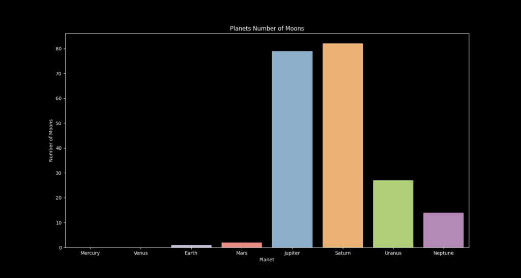
plt.figure(figsize=(15,8))
plt.style.use("dark_background")
sns.barplot(x = df['Planet'], y = df['Number of Moons'])
plt.ylabel('Number of Moons')
plt.xlabel('Planet')
plt.title('Planets Number of Moons')
plt.show()

plt.figure(figsize=(15,9))
plt.style.use("dark_background")
sns.barplot(x = df['Planet'], y = df['Diameter (km)'])
plt.ylabel('Diameter (km)')
plt.xlabel('Planet')
plt.title('Planets Diameter')
plt.show()

plt.figure(figsize=(15,8))
plt.style.use("dark_background")
sns.barplot(x = df['Planet'], y = df['Density (kg/m^3)'])
plt.ylabel('Density (kg/m^3)')
plt.xlabel('Planet')
plt.title('Planets Density')
plt.show()

plt.figure(figsize=(15,8))
plt.style.use("dark_background")
sns.barplot(x = df['Planet'], y = df['Surface Gravity(m/s^2)'])
plt.ylabel('Surface Gravity in (m/s^2)')
plt.xlabel('Planet')
plt.title('Planets Surface Gravity')
plt.show()

plt.figure(figsize=(15,8))
plt.style.use("dark_background")
sns.barplot(x = df['Planet'], y = df['Number of Moons'])
plt.ylabel('Number of Moons')
plt.xlabel('Planet')
plt.title('Planets Number of Moons')
plt.show()

plt.figure(figsize=(15,8))
plt.style.use("dark_background")
sns.barplot(x = df['Planet'], y = df['Mean Temperature (C)'])
plt.ylabel('Mean Temperature (C)')
plt.xlabel('Planet')
plt.title('Planets Mean Temperature (C)')
plt.show()

plt.figure(figsize=(15,8))
plt.style.use("dark_background")
sns.barplot(x = df['Planet'], y = df['Length of Day (hours)'])
plt.ylabel('Length of Day (hours)')
plt.xlabel('Planet')
plt.title('Planets Length of Day (hours)')
plt.show()

Links