Google Trends example using python

In this article we will look at grabbing some trends from google using their service which is of course called google trends

First of all you need to install the pytrends library

Installation

pip install pytrends

Requirements

• Written for Python 3.3+
• Requires Requests, lxml, Pandas

You can use the Google Trends web page or Pytrends library to get the following information

Interest Over Time
Historical Hourly Interest
Interest by Region
Related Topics
Related Queries
Trending Searches
Top Charts
Google keyword suggestions

Limitations

Searched terms and related topics are two different things, and the related topics sometimes don’t work at the place of related searched keywords
Google returns an error code when a keyword is greater than 100 characters
Google Trends shows the relative normalized data, and you can not use its data to estimate the exact amount of searches
You can query only five topics at a time

Code Examples

Here I will be analyzing the Google search trends on the queries based on “bitcoin ”, we will create a pandas DataFrame of the top 10 countries with the search term of “bitcoin” on Google

import pandas as pd
from pytrends.request import TrendReq
import matplotlib.pyplot as plt
trends = TrendReq()

trends.build_payload(kw_list=["bitcoin"])
data = trends.interest_by_region()
data = data.sort_values(by="bitcoin", ascending=False)
data = data.head(10)
print(data)

This is what I saw in the repl window when I ran the code above

bitcoin
geoName
El Salvador 100
Nigeria 77
Netherlands 49
Switzerland 49
Austria 47
Slovenia 46
Germany 39
Türkiye 38
Singapore 37
Cyprus 36

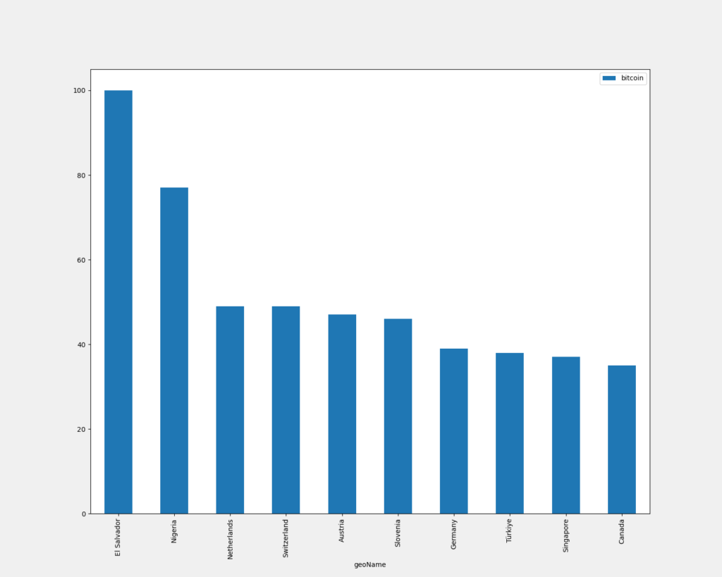
Now we will display this in a bar chart like this

import pandas as pd
from pytrends.request import TrendReq
import matplotlib.pyplot as plt
trends = TrendReq()

trends.build_payload(kw_list=["bitcoin"])
data = trends.interest_by_region()
data = data.sort_values(by="bitcoin", ascending=False)
data = data.head(10)
data.reset_index().plot(x="geoName", 
                        y="bitcoin", 
                        figsize=(15,12), kind="bar")
plt.style.use('fivethirtyeight')
plt.show()

And you should see something like this

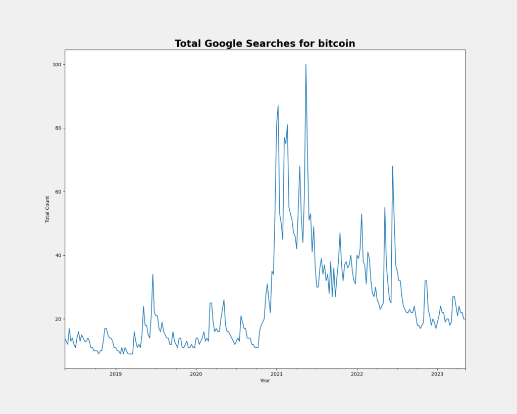
In this example we will display the search trend visually by year

import pandas as pd
from pytrends.request import TrendReq
import matplotlib.pyplot as plt
trends = TrendReq()

trends.build_payload(kw_list=["bitcoin"])
data = TrendReq(hl='en-US', tz=360)
data.build_payload(kw_list=['bitcoin'])
data = data.interest_over_time()
fig, ax = plt.subplots(figsize=(15, 12))
data['bitcoin'].plot()
plt.style.use('fivethirtyeight')
plt.title('Total Google Searches for bitcoin', fontweight='bold')
plt.xlabel('Year')
plt.ylabel('Total Count')
plt.show()

You should see something like this