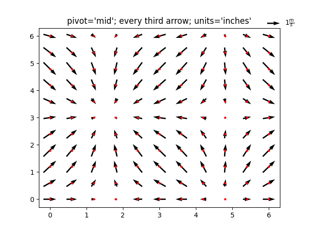
A matplotlib Quiver plot is a type of 2D plot which shows vector lines as arrows. Quiver(X,Y,U,V) plots arrows with directional components U and V at the Cartesian coordinates specified by X and Y.
The first arrow originates from the point X(1) and Y(1), extends horizontally according to U(1), and extends vertically according to V(1).
Syntax
matplotlib.pyplot.quiver([X, Y], U, V, [C])
Parameters
Where X, Y define the arrow locations, U, V define the arrow directions, and C optionally sets the color.
Arrow size
The default settings auto-scales the length of the arrows to a reasonable size. To change this behavior see the scale and scale_units parameters.
Arrow shape
The defaults give a slightly swept-back arrow; to make the head a triangle, make headaxislength the same as headlength. To make the arrow more pointed, reduce headwidth or increase headlength and headaxislength. To make the head smaller relative to the shaft, scale down all the head parameters.
Arrow outline
linewidths and edgecolors can be used to customize the arrow outlines.
| Parameters: |
|
|---|
Examples
Basic single arrow example
import numpy as np
import matplotlib.pyplot as plt


# Creating arrow
x_pos = 0
y_pos = 0
x_direct = 1
y_direct = 1

# Creating plot
fig, ax = plt.subplots(figsize = (11, 8))
ax.quiver(x_pos, y_pos, x_direct, y_direct)
ax.set_title('Quiver plot with one arrow')

# Show plot
plt.show()
Quiver Plot With 2 Arrows
import numpy as np
import matplotlib.pyplot as plt

# Creating arrow
x_pos = [0, 0]
y_pos = [0, 0]
x_direct = [1, 0]
y_direct = [1, -1]

# Creating plot
fig, ax = plt.subplots(figsize = (11, 8))
ax.quiver(x_pos, y_pos, x_direct, y_direct,
         scale = 4)

ax.axis([-1.5, 1.5, -1.5, 1.5])

# show plot
plt.show()
Other examples
import numpy as np
import matplotlib.pyplot as plt

X, Y = np.meshgrid(np.arange(0, 2 * np.pi, .2), np.arange(0, 2 * np.pi, .2))
U = np.cos(X)
V = np.sin(Y)

fig1, ax1 = plt.subplots()
ax1.set_title('Arrows scale with plot width, not view')
Q = ax1.quiver(X, Y, U, V, units='width')
qk = ax1.quiverkey(Q, 0.9, 0.9, 2, r'$2 \frac{m}{s}$', labelpos='E',coordinates='figure')

plt.show()
import numpy as np
import matplotlib.pyplot as plt

X, Y = np.meshgrid(np.arange(0, 2 * np.pi, .2), np.arange(0, 2 * np.pi, .2))
U = np.cos(X)
V = np.sin(Y)

fig1, ax1 = plt.subplots()
ax1.set_title("pivot='mid'; every third arrow; units='inches'")
Q = ax1.quiver(X[::3, ::3], Y[::3, ::3], U[::3, ::3], V[::3, ::3],pivot='mid', units='inches')
qk = ax1.quiverkey(Q, 0.9, 0.9, 1, r'$1 \frac{m}{s}$', labelpos='E',coordinates='figure')
ax1.scatter(X[::3, ::3], Y[::3, ::3], color='r', s=5)

plt.show()

![Java SE 11 Programmer II [1Z0-816] Practice Tests](https://static.shareasale.com/image/43514/728X9026.jpg)
![Java SE 11 Programmer I [1Z0-815] Practice Tests](https://static.shareasale.com/image/43514/728X909.jpg)

![Java SE 11 Developer (Upgrade) [1Z0-817]](https://static.shareasale.com/image/43514/728X9033.jpg)


